Literature Review: Selection on soil microbiomes reveals reproducible impacts on plant function

I recently found an intriguing microbiome paper, and I would like to post my thoughts about it.

Citation
Panke-Buisse et al., Selection on soil microbiomes reveals reproducible impacts on plant function, ISME Journal 2014, doi: 10.1038/ismej.2014.196.

Review
The main hypothesis in this paper tests if phenotypes from a soil microbiome connected with a single plant genotype can be recapitulated in other plant genotypes.  First, early- and late-flowering time associated soil microbiome were generated.  Ten generations of Arabidopsis thaliana Col-0 were grown and at each generation soils from the four earliest and latests flowering pots were collected as the inoculum for the subsequent generation.  Using soils from generation 10, final early- and late-flowering time associated inoculums were derived.  These inoculums were then administered to four Arabidopsis thaliana ecotypes (Rld, Ler, Be, and Col-0) and a close relative, Brasica rapa.  Flowering time, plant biomass, and nitrogen mineralization enzyme activity for each of the genotypes were statistically different between early- and late-flowering associated inoculum treatments except Ler (Fig 4).  Microbes specifically associated with early- and late- flowering time treatments were found in low abundance suggesting that low-abundance microbes can contribute significantly to interesting phenotypes.


Positives In general, I found this paper to be very insightful for the following reasons:

• Soil Microbial phenotypes can persist in novel hosts.  This is a really cool result and could have direct implications for building field-useful microbiome treatments.  However, flowering time is a well conserved phenotype so this result may not apply to other specific phenotypes of interest such as crop yield, disease resistance, or with greater host genetic divergence (i.e. corn flowering time vs arabidopsis).
• Low abundance members of a community can drive an important phenotype.  A common assumption in metagenomics is that the most abundant members of a community are the most important.  Perhaps more focus should be geared toward linking microbes to phenotypes regardless of abundance.
• This artificial selection design doesn't require detailed knowledge of genetic mechanisms in order to produce a desired phenotype.  It is similar to the old dogma of plant breading where two good plants were crossed to produce an even better plant with no underlying knowledge of the genetic mechanisms.  While understanding the mechanisms is important for maximizing the phenotypic benefits, it is not required to generate a positive effect.

Critiques and Questions

• The methods section seems incomplete.
• Why are there so few OTUs in the heatmap and ternary plot?  Were OTUs filtered out?  I would expect to see hundreds or even thousands of OTUs from soil-derived microbiota.
• Were the wild soils combined at equal ratios?
• What was their measure of flowering time?  I think there are well defined methods in the literature for observing flowering time.
• Why are the EF associated samples in the 10 generation experiment actually flowering at a later time in later generations (supp fig 1)?
• Why are the control samples not included in supp fig 1?  
• Even though control samples were included as a covariate to generate figure 4, I would have liked to have seen them graphed there as well.
• Perhaps a better way of generating the control samples would have been to randomly pick pots to generate a control inoculum.  This was what they did in Swenson et al., 2000

Future Work
This experimental design could be used to address the following intriguing hypotheses:

• Selection on soil microbiomes changes the root endophyte microbial community.
• Redo the experiment with the same design but also 16S profile endophyte microbes.  
• It would also be interesting to see if the microbes specific to each treatment are also found inside the root.  This would suggest a direct microbial effect on the plant phenotype.
• Selection for soil microbiome associated phenotypes is driven by multiple mechanisms.
• Redo the experiment but don't combine replicates such that the end inocula include four independent lines of selection for both early- and late-flowering time soil microbiomes.  Compare microbes among treatment groups looking for different microbial profiles that express similar phenotypes.  

MiSeq Flow Cell Edges Correlate with Low Quality Scores

Upon receiving a FASTQ file fresh off the MiSeq, the first question I ask myself is:  "Did the sequencing work?"  On several occasions I open these files to discover the first few pages of sequence reads are littered with N's and have low quality scores.  However, when I run the full set of reads through a QC pipeline (e.g. FastQC) an overwhelming majority are high quality.

So why is it that the reads at the beginning of the FASTQ file have such poor quality?

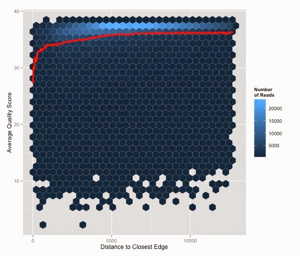
Reads generated using Illumina technology are ordered by their cluster's y-coordinate on the flow cell.  This led me to hypothesize that clusters near the edge of the flow cell are more likely to have low quality scores.  To test this hypothesis I took a subset of reads (932,709) from a MiSeq run, calculated their average quality score, and graphed that against the distance from the closest edge.

The splines function in R was used to model the relationship between average quality score and distance from the closest flow cell edge (red line).  Clusters closer to the edge of the flow cell have significantly lower quality scores.  However, the good news is that the vast majority of clusters do not fall close to the edge (light blue heat).  

In practical terms this issue is insignificant because so few reads are affected, but it does explain the high concentration of low quality reads at the beginning (and end) of Illumina generated FASTQ files.

When is my genome finished?

This is a common question for anyone doing genome sequencing and assembly.

The short answer:  never.

The slightly longer answer:  it depends.

The long answer:  Finishing a genome means the order of all nucleotide bases have been correctly resolved.  Even for simple genomes this is extremely difficult.  Billions of dollars have been spent to sequence the human genome, and it is currently estimated that 92% of the human genome has greater than 99.99% accuracy (Schmutz et al., 2004).  In total, 99% of the genome has been assembled, and the remaining 1% are likely to be highly repetitive regions with little or no gene content (remember that 1% of 3 billion total bases means there are about 30 million unresolved bases).  Using the current technology, it is impossible to reach 100% accuracy across 100% of the human genome.  For simpler genomes such as some viral and bacterial genomes it is possible to completely resolve the entire sequence.  However, because these genomes are much more dynamic (i.e. change at a faster rate), generating a completely finished genome may not be worth the cost.

Finishing a genome requires a substantial amount of time, work, and money.  However, getting a genome to draft status (i.e. incomplete but usable) can be done with minimal costs and resources.  So perhaps the most important question is:  when is my genome usable?  The answer to this question depends on the research questions being considered.  For example, when studying the evolutionary history of genomes with a high propensity for genomic rearrangements, generating long contigs/scaffolds is important for determining the orientation and lineage of genomic rearrangements.  Alternatively, some research questions are more concerned about the completeness of the gene content for making functional comparisons between genomes.  For such a question, generating long, continuous contig/scaffolds is less important.

Here are some possible ways to estimate completeness (with what I think are the best methods near the top):

• Compare the gene content of highly conserved genes
• Eukaryote:  CEGMA
• Bacterial:  CheckM
• Archaeal:  A table of 53 conserved COGs
• Check for possible errors using REAPR
• Calculate assembly metrics like contig number, N50, coverage, and assembly size.  
• Compare the size of your assembled genome to a related (or set of related) genome(s).  

See these papers for interesting discussion on evaluating assemblies:  

• Salzberg et al., 2011.
• Vezzi et al., 2012.
• Gurevich et al., 2013.
• Shangguan et al., 2013.
• Pan et al., 2014.

How to Order Contigs Using a Reference Genome

Background
In genomics complete (i.e. finished) genomes provide an excellent resource for future sequencing projects.  However, generating finished genomes is an expensive and laborious endeavor.  In some cases, the returns of finishing a genome are not worth the cost particularly when draft genomes can provide enough information for robust hypotheses testing.  Draft genomes contain a large number of unordered sequences of various lengths called contigs.  Contigs can be joined into more contiguous sequences called scaffolds using paired-end reads.  While a set of contigs/scaffolds can be useful for a wide variety of projects (gene annotation, gene expression profiling, etc.), contig order provides vital information in comparative genomics and analyses of specific genomic regions.  Typically, a rough ordering of contigs can be accomplished by mapping contigs to a closely related reference genome.

ABACAS
Recently, I discovered a nice software package called ABACAS which not only orders contigs but creates a contiguous sequence representing the connected contigs.  Gaps between contigs are represented by N's and overlapping regions are resolved (although I could not find information on exactly how).  Because ABACAS requires MUMer, its outputs integrate will with other MUMer scripts such as those for visualizing alignments (Figure 1, i.e. mummerplot).  ABACAS is hosted by SourceForge and is well documented.  It was published in Bioinformatics in 2009.

Notes
Of course, more closely related draft and reference genomes will generate the most correct ordering.  However, in cases where the target genome is VERY closely related to the reference genome it may be better to map raw reads to the reference genome instead of build a de novo assembly.  Deviations from the reference genome can be discovered using SNP detection software.  Read mapping experiments are generally cheaper because they require fewer reads than de novo assembly but can still detect biologically significant differences when compared to the reference genome.

Cool Unix Commands

I will add to this list as I discover new ones.  If you have a favorite or useful command feel free to include it in a comment on this post.

Convert a FASTQ file to FASTA (originally posted here):

sed -n '1~4s/^@/>/p;2~4p' 

NOTE: this assumes that each FASTQ entry spans only four lines as is customary.



Convert a SAM file to FASTA

awk '{OFS=""}{print $1, "\n", $10; }' file.sam > file.fasta

NOTE: You will loose a lot of information in the sam file.  You can save more of that info by adding column variables to the print statement.  Also, you may have to change the column variable numbers depending on your sam file format.  This is just a general example.



Replace spaces in file names with underscore (originally posted here)

rename ' ' '_' *

NOTE:  do NOT put spaces in file names!!  This is so annoying!



Get a histogram of sequence lengths from FASTA/Q files (from Surge Biswas)

FASTQ:  cat <fastq file> | awk '{if(NR%4==2) print length($1)}' | sort -n | uniq -c
FASTA:  cat <fasta file> | awk '{if(NR%4==0) print length($1)}' | sort -n | uniq -c



Do arithmetic operations on the bash command line

echo $((1 + 1))
echo $((1 - 1))
echo $((1 * 1))
echo $((1 / 1))
echo $(((1+3) / (1+1)))

For floating point operations you can use the bc tool.  For example

echo "scale=1; 1/2" | bc



Add a comment to a bash command on the command line

<command>; # this is a comment line

A practical example:  mv file1 old_file1; # there is now a new file1 is a more recent version

NOTE:  Do you ever have a long and complex command for which you would like to save a simple note?  You can use this little trick and the note will be saved along side your command in your history.  The next time you look through your history to rerun the command you will also see the associated note.



Count the number of bases in a FASTA file

grep -v ">" file.fasta | wc | awk '{print $3 - $1}'

(from martinghunt on SEQanswers)

How to Learn Bioinformatics

Introduction

At least once a month someone asks me for help learning bioinformatics.  I love it when this happens because it usually means they want to take control of their own analysis thereby freeing up my time for problems that interest me.  This post is a collection of tips and resources for people wanting to learn how to do bioinformatics.

Keep These Things in Mind:

• Learning the basics of bioinformatics is easy.  The basics as described in this post are often taught in high school.  However, don't get frustrated if you don't understand everything all at once.  Learning anything new takes time and practice no matter its difficulty.  
•  A little bit goes a long way.  I estimate that nearly 90% of my work is occupied by simple routine procedures.  Learning how to do these tasks will substantially expand your ability to analyze and interpret your data.
• Google it.  Google is the best resource for learning new techniques and trouble shooting problems.  If you have a question type exactly what you would say to a person into the google search bar.  When you take questions to your bioinformatics friends it's likely they won't know the answer offhand and will google it anyway.
• Try it.  If you're not sure about something try it and see what happens.  Generally, there is very little danger is just trying a command to see if and how it works.  That being said it's a good idea to backup important files and data just incase something goes very wrong.  Every Unix programmer that I know has deleted a really important file using the rm command (which is one of the few irreversible Unix commands).  It's going to happen to you too so make a backup.

Learn the Unix Basics

• Get on a Unix machine.  Doing is the most important aspect of learning Unix.  You will never fully understand the basic concepts if you only read about them.  Mac users have it easy because OSX is build on a unix shell.  Simply open the terminal application and you are ready to start with an online tutorial.  For non-mac users I recommend finding an old computer and installing a Linux/Unix operating system like Ubuntu.  A slightly more difficult approach would be to partition the drive of an existing computer to dual boot a Linux/Unix OS along with the existing OS.
• Complete an online tutorial
• Unix Tutorial for Beginners
• Introduction to Unix for Biologists
• Unix and Perl Primer for Biologists

• Buy a book if you are a book learner.  However, the basic can pretty much all be learned using online materials.  My favorite Unix book is O'Reilly's Unix Power Tools.

Learn a Scripting Language

• Pick a scripting language.  Scripting languages are computer languages that are not compiled (i.e. they are interpreted by the computer on the fly).  The two most popular bioinformatics scripting languages are Perl and Python.  Both languages have their strengths and weakness, but I personally prefer Perl.
• Complete an online tutorial for your language.
• Perl tutorial
• Perl and Unix for Biologists
• Python tutorial
• Python for Biologists
• Buy a book.  My favorite Perl book is Perl Best Practices by Damian Conway.  This book is a must have for all Perl programmers!  I don't have much experience with Python books, so I would recommend looking at book reviews before making a purchase.

Learn a Statistical/Graphing Language

• Pick a language for doing statistical operations and building figures.  Languages like R and Matlab are prime choices for both statistics and graphics.  Both languages have their strengths and weaknesses, but I personally prefer R.  If you choose R I highly recommend using the ggplot2 library for building figures.  
• Complete an online tutorial for your language.
• R tutorial (ggplot tutorial) (another fantastic R tutorial by DataCamp)
• Matlab tutorial 
• Give up Excel.  Excel is a powerful program but lacks the flexibility of computer languages like R and Matlab.  While there is a steeper learning curve for R and Matlab, you will substantially enhance your ability to do statistical analyses and build graphics by getting away from Excel.

Learn Basic Bioinformatics Procedures and Corresponding Software Tools

For example:

• Quality control
• fastQC
• Sequence assembly
• Velvet,
• SPAdes (my preference, also see this post)
• Sequence mapping
• BWA
• Bowtie
• Sequence searching
• BLAST
• Differential expression
• edgeR
• DESeq
• Variant calling
• GATK
• etc

This is only a small list of procedures and tools primarily focusing on DNA sequence analysis.  For a more comprehensive list see OMICtools.


Find a problem

I strongly encourage new bioinformaticians to find some real data to do meaningful science using the above principles and skills.  If you don't personally have data I recommend downloading data from a public repository (i.e. Genbank).  A similar alternative would be to choose a paper that uses a procedure you are interested in learning and recapitulate the results.  

Predicting Full-Length Ribosomal Gene Sequences

Introduction

The 16S ribosomal gene has been used extensively in biology for distinguishing relatedness between species.  This gene has regions of DNA that are highly conserved among almost all living organisms and other regions that have high DNA sequence variability.  The conserved regions are ideal for building PCR primers that can amplify DNA from many different organism.  The variable regions that are amplified using these conserved primers can be used to determine the relatedness between two or more organisms.  Closely related species typically have much more similar DNA sequences than distantly related species.

Typically PCR is used to amplify a portion of the 16S ribosomal gene for sequencing.  However, whole genome sequences or whole metagenome sequences also contain short DNA reads originating from the 16S gene.  These reads can be separated from the pool of other genomic reads and assembled into the entire 16S gene.  EMIRGE (Miller, et al. 2011) is an algorithm for reconstructing full-length ribosomal genes from short read DNA sequences.


EMIRGE

EMIRGE reconstructs full-length ribosomal genes from short read DNA sequences.  It first maps reads to a database of known 16S genes such as the SILVA or greengenes database.  After the initial mapping, EMIRGE estimates the probability that a given read was generated from the reference to which it mapped.  Based on these probability estimates, reference sequences are changed to reflect the 16S sequences that are likely to be represented by the set of reads.  Reads are then remapped to the adjusted 16S sequence database and the processes is repeated until an equilibrium is achieved.  The resulting database of 16S sequences reflect the likely 16S genes represented by the input set of short reads.

This software was primarily built to infer the set of 16S genes from whole metagenome reads.  However, it can also be used to infer the single 16S gene from genomic sequences from a single isolate.  Full-length 16S genes are difficult to assemble even when only reads from a single genome are considered.

In the Dangl lab, we use EMIRGE to predict full-length 16S genes from reads generated from a single genome of bacteria.  An example of the EMIRGE command we use is:

emirge.py my_output_dir -1 fwd_reads.fastq -2 rev_reads.fastq -b SSURef_NR99_115_tax_silva_formated -f SSURef_NR99_115_tax_silva_formated.fasta -i 600 -s 1000 -l 250

The descriptions of each parameter are below:

my_output_dir: the output and working directory for EMIRGE.

-1: the forward or single-end genomic sequencing reads

-2: the reverse end genomic sequencing reads

-b: the bowtie index of the 16S sequence database

-f: the fasta file of the 16S sequence database

-i: insert size of paired-end reads

-s: standard deviation of insert size for paired-end reads

-l: max length of reads


Other Details

EMIRGE uses bowtie to map reads to the reference database.  To build the bowtie index of the reference database the following command was used:

bowtie-build SSURef_NR99_115_tax_silva_formated.fasta SSURef_NR99_115_tax_silva_formated

Also, the database downloaded from SILVA had to be reformatted using this Perl script.  This script requires BioUtils.

2014 JGI Users Meeting Notes

Here are some notes from a few of the speakers at the JGI Users meeting in California.  In general the speakers were fantastic.  Some general themes of the conference include:  single-cell genomics, synthetic biology, fungal metagenomics, and metabolics.  A person take-home message for me was the need for creative biological solutions to common issues that the human race currently faces or will face in the near future.

Mark Ackermann (opening keynote) – A Single Cell Perspective on Bacterial Interactions

- Focused on phenotypic heterogeneity, when identical cells have different functional profiles.

- Most genes don’t have clonal variation but in the ones that do how is that heterogeneity important for the community.

- Salmonella is an example of phenotypic heterogeneity.  One cell type causes inflammation and one uses the inflammation response to reproduce and cause full infection.

- Different cell types survive better in different environmental conditions.

- Another example of phenotypic heterogeneity is in alpine lakes where there are generally large amounts of ammonium that bacteria can use as a nitrogen source.  However, there are some cells that fix their own nitrogen in the event that ammonium runs out.

- preliminary data show that neighboring cells are more likely to be of the same cell type.

Mary Berbee – Pectinases link Early Fungal Evolution to the Land Plant Lineage

- Sequenced early divergent fungal groups.

- The relationship between the early branching groups is still poorly resolved.

- Showed some cool trees where she had overlaid two trees to highlight difference between the two.  I would like to know what software she used to do this.

- Her trees were based on whole genomes but I’m not sure how she built them.

Rytas Vilgalys – Understanding the Forest Microbiome:  A Fungal Perspective

- Oak and pine share many fungi while populus has more different fungi.

- Soils from the same region are likely to share the same fungi.

- Populus of different genotypes do not assembly different fungi.  At least not nearly as different as fungi from different regions.

- They have isolated ~1,800 fungal isolates.  These isolate represent only ~15% of the isolates that are likely populus endophytes.

- Many fungal isolates stimulate plant growth.

- They are re-inoculating these isolates to confirm they are endophytic.

- Mortierella elongata is an isolate that stimulates plant growth in populus and Arabidopsis thaliana.

- M. elongata also harbors bacterial symbionts (Glomeribacter which are known to affect lipid fermentation and is a sister to Burkholderia.  These bacteria cannot be cultured possibly because they rely so heavily on the host for nutrients). 

- M. elongata migrate to the roots.

- Different genes are expressed in M. elongata grown in culture than those sampled from the rhizosphere.

- Different genes are expressed in M. elongata inoculated on different hosts.

Eddy Rubin

- Bacterial genes are typically ~900bp.

- In a couple of sequenced genomes they saw average bacterial gene lengths as low as 200bp.  However, when they adjust the codon table by replacing one of the stop codons to code for a glycine predicted genes have an average length of 900bp!  Some bacteria use different codon translations! 

- Natalia Ivanova is a gene annotation specialist they consulted for help in this analysis.

- They found evidence of recoding in lots of other bacteria by looking at sequenced isolates.

- Didn’t find evidence of recoding in archea. 

- They show that phages which use different codon profiles can circumvent host cell machinery to match their codon profile!

- CRISPR regions in bacterial cells often contain phage elements that correspond to different codon profiles.  This is further evidence that phages with different codon profiles can infect cells with canonical codon profiles. 

Nicole Dublier –Metagenomics and Metaproteomic Analyses of Symbioses between Bacteria and Gutless Marine Worms

- Bacteria can use hydrogen to produce more energy than methane.  Nature 2011

- They discovered key genes able to metabolize hydrogen.

- The second half of the talk was about gutless worms living in shallow water.  They completely dependent on bacterial symbionts for feeding and waste excretion. 

- There are species specific symbionts.

- Her proteomics data yield more obvious features than comparative genomics.  As an example she shows how one isolate contains a protein that does the function of 3 different proteins in the canonical Calvin Cycle.  DNA sequencing confirmed this observation but would have been a “needle-in-a-haystack” for a comparative genomics project.  This work published in PNAS.

Erin Nuccio – Mapping Soil Carbon from Cradle to Grave:  Using Omics and Isotope Analyses to Identify the Microbial Blueprint for Root-enhanced Decomposition of Organic Matter.

- The general question is how do microbes transform and stabilize root carbon in soil.

- Carbon can affect nitrogen rates.

- Plants fix carbon for microbes in the soil.

- Looking at the rhizosphere over time it gradually deviates from bulk soil in carbon levels at time points of 3, 6, 9, and 12 weeks.

- Some preliminary data show that bacteria prefer carbon excreted by plant over as an energy source over nitrogen liter material (ie material artificially added to the system).

Michael Fischbach – A Gene-to-Molecule Approach to the Discovery and Characterization of Natural Products

- Discovers natural gene products.  By gene products I think he means functional protein units.

- Undiscovered gene products are often coded by clusters of genes.

- Has some type of algorithm to computationally discover these clusters that may produce unknown gene products.

- Lots of his most interesting clusters were found on human associated microbes.

- Discovered several oligosaccharide clusters.  These bacteria were very difficult to work with but these clusters and the functions they provide to the human host are of high interest.

- The general observation of this study was that microbes in our gut are making products for which we have no idea what they are or how they function.  It’s like taking several prescription drugs for your entire life!  We need to figure out what is going on in there. 

Kelly Matzen – Genetic Control of Mosquitoes

- In the 50’s DDT was used to control mosquito populations and subsequently mosquito born disease such as dengue.  However, DDT is know to be detrimental to the environment in several ways and therefore is being used much less.  We are starting to see diseases like dengue make a comeback in places like Florida and of course in places like Central and South America.

- Right now the most effective control is pesticides. 

- They are releasing massive numbers of sterile male mosquitoes to control (ie reduce) mosquito populations.  This technique has been successfully used before in the United States to control populations of other insects many years ago.

- This technique seems to be working in the small field studies they have been conducting. 

- There is some push back from legislators but in general it seems like good solution.

Cameron Coates – Characterization of Cyanobacterial Hydrocarbon composition and Distribution of Biosynthetic Pathways

- Cyanobacteria produce over 30% of the earth’s oxygen.

- They are very diverse and live in all sorts of habitats on earth.

- They can produce hydrocarbons where are relevant of use of biofuels.  However, they don’t produce large amounts of hydorcarbons.

- They looked at the evolution of cyanobacteria hydrocarbon pathways.  There are two main pathways.  Several clades have both pathways suggesting a large amount of horizontal gene transfer. 

- This work was published in PLOS ONE.

June Medford – Making Better Plants:  Synthetic Approaches in Plant Engineering

- They created a biological input/output system.  This allows for some external factor to cause a reaction that can be observed in the plant.

- They use a pariplasmic binding protein as the input signal because it can quickly defuse through the cell wall and are then translocated to the nucleus to transcriptionally regulate some response. 

- They can theoretically use this system as a flag for pollutants or other dangers that we currently use very expensive technology to detect.

- They are currently developing a system to detect TNT where the response signal of the plant is to turn white.  This system can detect traces of TNT 10x smaller than a dog!  There are still some kinks to work through like response time.  But looks like a very promising system.  This idea has countless unexplored applications!

Kankshita Swaminathan – Genome Biology of Miscanthus

- Miscanthus is in the same clade as sugar cane, corn, and sorghum.  These plants have been amenable to breading.

- The genomic sequence of sorghum is very close to Miscanthus except that Miscanthus has had a whole genome duplication event.

- In the winter all the nutrients migrate to the rhizome leaving only the stalk above ground.  The stalk is the most important element for biofuels and can be harvested without significantly depleting soil nutrients.

Annalee Newitz (closing keynote) - How Humans Will Survive a Mass Extinction

- Humans have a very good chance of surviving a mass extinction because we are very adaptable.  However, our focus should be how we can preserve the diversity of the earth as it is now.

- A mass extinction is when greater than 70% of the earth's species are killed.

- Five mass extinctions have occurred in the history of the earth.  Perhaps the largest was caused by cyanobacteria because they released large amounts of oxygen into the atmosphere.  Close to 90% of species became extinct as a result.

- Climate change is inevitable regardless of wither or not humans are the cause.

- The questions we should be asking are:  how can we respond to these changing climates and what can we do to preserve the world as we know it.

- Space travel seems like an important step in human survival.  

The Pan/Core/Accessory Genome

Introduction
The term "pan genome" was coined in 2005 by Tettelin in a paper describing the genomes of eight pathogenic Streptococcus strains.  The pan genome is the set of all unique genes from a set of genomes (ie gene union).  The core genome is the set of genes found in each genome (ie gene intersection).  The accessory genome is the genes unique to a particular genome (ie strain specific genes).  

Previous Studies
Read et al. (2012) discusses the pan and core genome of phytoplancton.  They estimate the size of the E. huxleyi pan genome to be large because there are several thousand genes in the reference that are missing from all of the three well-sequenced isolates.  This is definitely more of a core genome paper (the analysis of which is easy when you have a reference).  Perhaps a better way of showing the diversity of the pan genome is rarefaction curves on the number of homologous genes or perhaps k-mer content.  The lead investigator, Igor Grigoriev, is the fungal genomics lead investigator at the JGI.

Pan and Core Genome Dynamics
In general, as more genomes are added to the analysis set, the core-genome shrinks and the pan-genome grows.  Collins (2012) describe these dynamics in their Molecular Biology and Evolution publication by using an infinitely many genes (IMG) model.  In summary, the Collins IMG model is based on the idea of three types of gene classes:  core, shell, and cloud genes.  Core genes are those found in all genomes, shell genes are gained and lost from genomes at a relatively slow rate, and cloud genes are rapidly gained and lost from genomes.  Empirical data from a set of Bacillaceae genomes support the Collins IMG model.  The Collins IMG model can be used to predict the size of core- and pan-genomes.  In the Dangl lab this has become a question of substantial interest for determining which relevant clades require more isolate genomes for more robust functional genomics analyses.

Core vs Accessory
Given a set of genes from various genomes what gene set is most interesting?  Of course this question will most heavily depend on previous knowledge of the genomes in question.  In the Dangl lab we are interested in microbes that inhabit the endosphere (inner plant root).  Because the set of microbes living inside these roots exhibit a different profile than surrounding soil, one could hypothesize that a single or small set of genes are responsible for a microbes ability to inhabit the inner root.  Under this hypothesis the core-genome would be of particular interest because it should contain these genes.  However, in practice the core genomes is primarily composed of common cellular functions ubiquitous to all bacteria.

Because the core-genome is likely to reveal nothing of specific interest the accessory-genome seems most interesting.  The genes in this set alludes to what makes a particular genome functionally distinct and interesting.  They get at questions like:  "What functions does a particular bacteria provide to the community."

Software for pan-genome analysis
The primary aim in any pan-genome analysis is grouping orthologous genes from different genomes.  To do this many pan-genome pipelines utilize algorithms and databases such as GO, COG, KEGG, eggNOG, Pfam, etc.

Here are some notes on various pipelines developed for pan-genome analyses.

• GET_HOMOLOGUES (my recommendation)
• This is my program of choice for pan/core/accessory genome analyses.  
• Fantastic documentation
• Options for bidirectional blast hit (BDBH), COGtriangle, and/or orthoMCL algorithms for building clusters of orthologous groups.
• Builds clear figures
• Several options for powerful downstream analyses. 
• Parallelization options
• Panseq (Laing, 2010)
• Nice web-based interface.  
• Seems to work (as opposed to some of the following programs)
• Output formats are not as user friendly or as concise get_homologues
• Job completion email never comes in.  Be sure to save the link somewhere.
• More suited for small, quick analyses
• PGAT (Brittnacher, 2011)
• Nice web-based interface and documentation
• Limited to comparisons between only a small number of genomes already stored in their database. 
• PGAP (Zhao, 2011) 
• Did not install because it requires the old version of blast (blastall)
• PanFunPro (Lukjancenko, 2013)
• Still in the development stage.   I had a quick look at the source code and there were some things didn't make sense.  I'll give the developers a little more time to work out the kinks.  
• The installation can take some time because of some large dependencies (eg. InterProScan).  Furthermore, the installation for the PanFunPro Perl scripts could be streamlined using a tool like Module::Build.  However, the installation instructions for it's dependencies are well written making installation remarkable easy. 
• PanOCT (Fouts, 2012)
• Primarily an algorithm for determining homology between a set of genes from 2 or more eukaryote genomes.  
• Considers conservation of neighboring genomic regions for determining homology.  The basic idea is that two genes are truly homologous (as opposed to paralogous) will be situated in the same genomic location.

A Brief Introduction to Sequence Assembly

Assembly Background

Sequence assembly is one of the overarching challenges in bioinformatics.  To understand the assembly problem it helps to understand some basics of DNA sequencing.  Consider a bacterium having a genome comprised of a single 5 megabase (5 million base pairs) chromosome.  Ideally, sequencing machines would start at the beginning of the chromosome and read each of the 5 million base pairs until arriving at the end.  Unfortunately, the current technology is limited to reading sequences between 30 and ~10,000+ bases.  The assembly problem is to take these short segments of DNA called reads and overlap them in such a way to recreate the original 5Mb chromosome.

To illustrate this consider the set of character strings below that come from a quote by Theodore Roosevelt (spaces have been replaced with "_" for clarity).  Can you put the pieces together to find out what it says?

You should end up with something that looks like this:

This is more or less what assembly programs attempt to do with DNA.  Some things to notice in the above example:

• Repeats can be problematic during assembly.  Notice that the word "you" is used twice in this sentence.  Looking at the two character strings "Believe_yo" and "you're_ha" you may have incorrectly merged them to form the character string "Believe_you're_ha" which is an incorrect assembly.  DNA repeats are common in genomes and can fragment assemblies or cause assembly mistakes.
• Longer reads can help with the repeat problem.  For example, given only two long character strings "Believe_you_can_and_you're" and "can_and_you're_halfway_there" it is much easier to unambiguously assembly the quotation despite the fact that the word "you" is used twice.
• Sequencing errors complicate assembly.  For example, if the character string "halfway" was sequenced as "calfway" there would be no way to finish the assembly correctly because "you're_ha" does not overlap with "calfway."  
• Coverage (i.e. the number of times a character is represented in the assembly) helps distinguish sequencing errors.  For example, if we sample from the quote (or in the genome in the case of DNA) many times and see the character string "halfway" 100 times and the character string "calfway" only once we can assume that "calfway" was incorrectly sequenced.  

De Novo vs Mapping Assembly

De novo is a latin expression meaning "from the beginning" (Wikipedia).  De novo sequence assemblies are build with no external information beyond the raw sequencing reads.  First pass de novo assembles are called "draft" assemblies because the genome remains fragmented (i.e. discontinuous) and may contain assembly errors.  Extensive resequencing and curation is generally required to "complete" or "finish" a genome assembly.

Alternatively, mapping assembly uses a reference sequence as an anchor to orient sequenced reads.  After reads are ordered based on their location in the reference sequence a consensus sequence is generated from all the mapped reads.  The consensus sequence can differ from the reference sequence but differences are generally single base differences scattered throughout the genome.  Mapping assembly is most useful when the reference sequence and sequenced organism are closely related.

In some cases (e.g. metagenomics), a combination of de novo and mapping assemblies may be advantageous.  However, hybrid assembly algorithms and protocols are not well explored.

De Novo Assembly Algorithm Classes

There are two main classes of assembly algorithms used in de novo assembly:  overlap-layout-consensus (OLC) and de bruijn graph (DBG).  Similar to the above example, OLC first finds reads with overlapping ends, builds a layout graph based on these overlaps, and lastly generates a consensus sequence as the graph is traversed.  OLC was the first assembly method developed and works well with long-read, low-coverage sequencing technologies like Sanger (and possibly PacBio).

DBG based assemblers convert the set of reads into a set of k-mers (i.e. short DNA sequences of length k).  These k-mers are then used to build a de bruijn graph from which the genomic sequence is inferred.  DBG assemblers work well with high-coverage sequencing methods like Illumina and Ion Torrent.  

Useful Links

• For more information and comparisons between OLC and DBG see this review.
• What is finished and why do we care? (Genome Research 2002).
• A review of assembly algorithms including:  SSAKE, SHARCGS, VCAKE, Newbler, Celera Assembler, Euler, Velvet, ABySS, AllPaths, and SOAPdenovo (Genomics 2010).
• How to apply de bruijn graphs to genome assembly (Nature 2011).